Intro to Bayesian Optimization 2. The Bayesian Optimization Framework

This is the second part in my Intro to Bayesian Optimization

1. Optimization Intuitions
2. The Bayesian Optimization Framework
3. Intro to Bayesian Statistics
4. Gaussian Processes

Random Search is widely used, especially when you have a lot of resources you can use in parallel. However, the expected number of samples required to find a good solution can grow with the number of dimensions and size of the “good” section of the sample space.

But what if you can’t do things in parallel, and what if sampling is expensive or limited. In practice, we can often only sample our experiments a few times due to resource constraints, so we want to get the most bang for our buck and learn as we go.

Bayesian Optimization offers a very practical way to approach optimization in experimental setups where running an experiment takes significant time and/or resources, and the experiments are done iteratively instead of all in parallel. Compared to grid/random search, think of it as getting the same information in fewer experiments, or getting more information from the same number of experiments.

When do we use BO

$$\begin{array}{c}\arg \underset{x}{\max }f(x)\end{array}$$

• Global optimization: We want to find the global (not local) optimum of some function $f$ (in the bounds that you provide)
• Continuous: there shouldn’t be any discontinuous jumps in $f$ from a small change in $x$ (this is usually an assumption we make if we don’t know a reason why that wouldn’t be the case)
• Black box: We don’t know the function $f$, and we don’t know any special features of $f$ like it being linear or concave
• Sequential sampling: We can sample $f$ where we choose, and we sample one point at a time (batch methods have been developed as extensions)
• Derivative-free: We cannot sample the first or second-order derivatives of $f$, otherwise we would choose gradient methods
• Expensive: $f$ is expensive to evaluate at each sample (high computation/high resource/limited samples)
• Not-too-high-dimensional: $x$ is at most 20 dimensional (e.g. we are looking at combinations of at most 20 cookie ingredients). This is more a rule of thumb
• Simple constraints: The bounds of $x$ are simple, we can describe it with a hyper-rectangle or $n$-dimensional simplex (e.g. the range of each ingredient is independent, or the sum of proportions is 1)

It turns out this combination of properties appears all the time in experimental design.

BO strategy

Given we don’t know $f$, we are going to construct a model for the function. We do understand the model, so even if it’s not 100% correct, we can still find its optimal value. Think about it as fitting a regression to the observed points. We will cover this in the next section, but this must be a Bayesian regression, and usually, we use a Gaussian Process. Compare this to the methods in the previous section where none of the approaches involved constructing a model.

Our goal is then to improve the model as much as we can through information we acquire via sampling. If we have a notion of uncertainty in the model, we can do this intelligently.

Using the model, we construct an acquisition function that tells us the next best point to sample. This point won’t just be the point that maximizes the model, it aims to direct our sampling to points that decrease the uncertainty of the model while searching areas that we believe have good solutions.

Note, in the literature, the name for the model in Bayesian Optimization is a surrogate model. That is because the main application for BO is in machine learning hyperparameter optimization. Our experiments may involve us sampling some point of parameters in the real world, but in hyperparameter optimization the experiment would be training the ML model for a given set of hyperparameters. So surrogate model refers to the cheap to evaluate model of an expensive to train ML model.

BO Algorithm

1. Start with some initial sample measurements
2. Fit a probabilistic model to the data
3. Compute the acquisition function based on the model
4. Find $x^{\ast }$ that maximizes the acquisition function
5. Sample $f(x^{\ast })$ and add to your data
6. If time/resources are remaining, go to step 2

BO Example

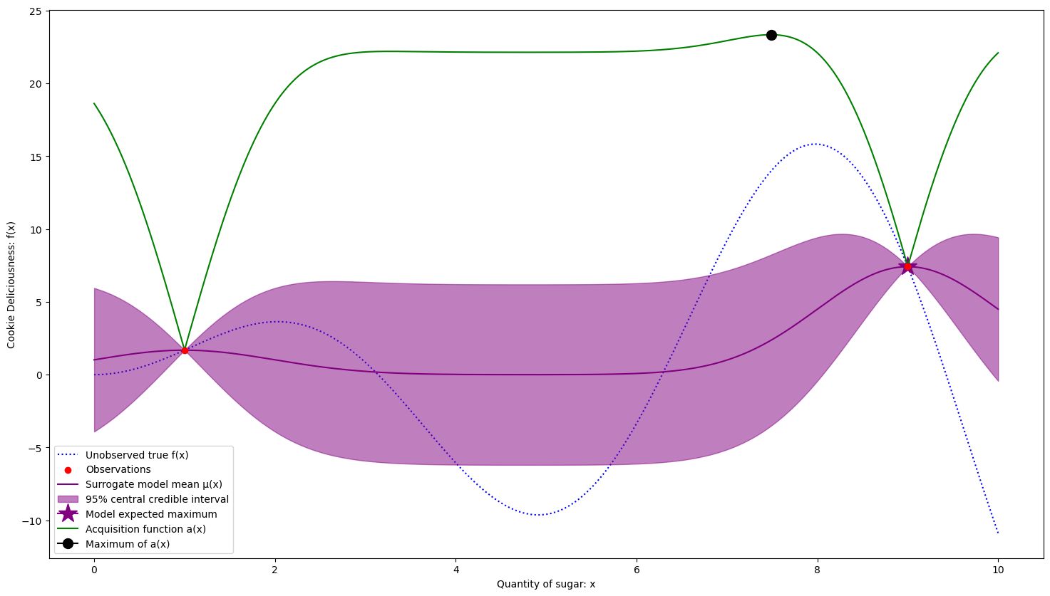
Starting samples at $x=1$ and $x=9$

The first suggestion is given at the maximum off the acquisition function, close to our best found solution but further to the right to capture some noise (wide purple area)

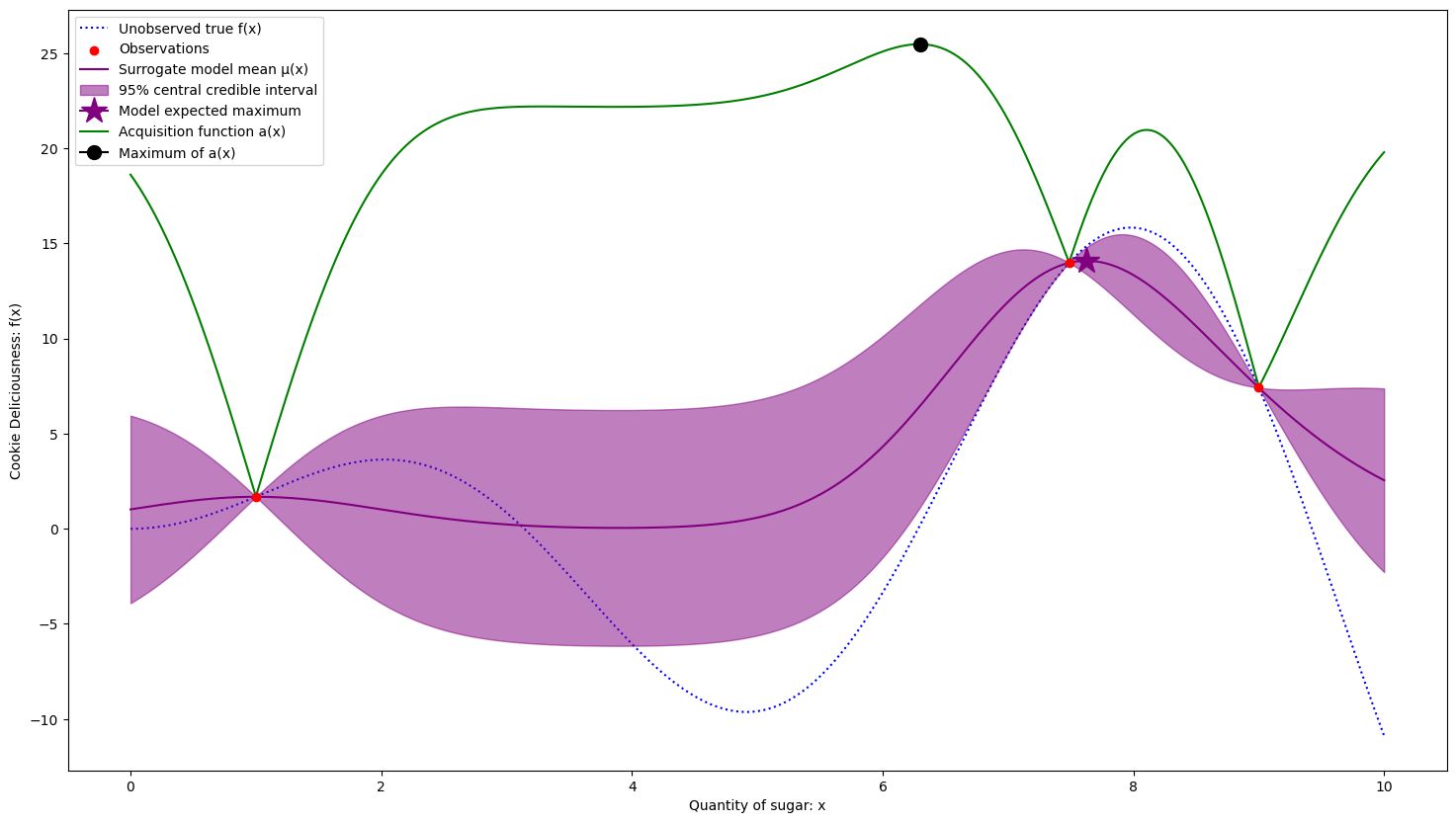
3 samples. The acquisition function is moving towards an expected worse section off the search space because it is favoring noise

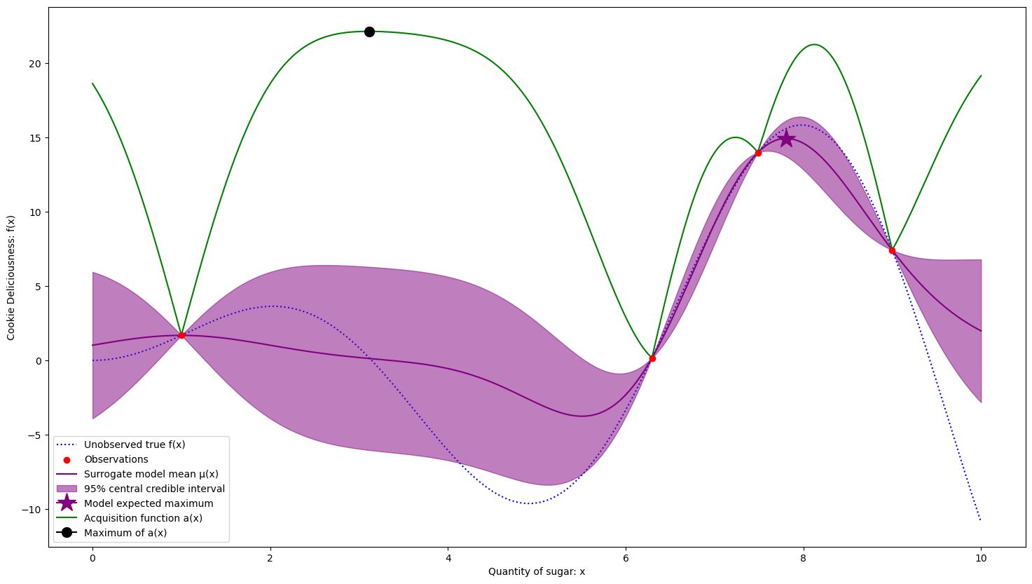
4 samples. The acquisition function is taking us to an underexplored area of the search space.

5 samples. The exploration has not been fruitful, so it is returning to a higher expected area.

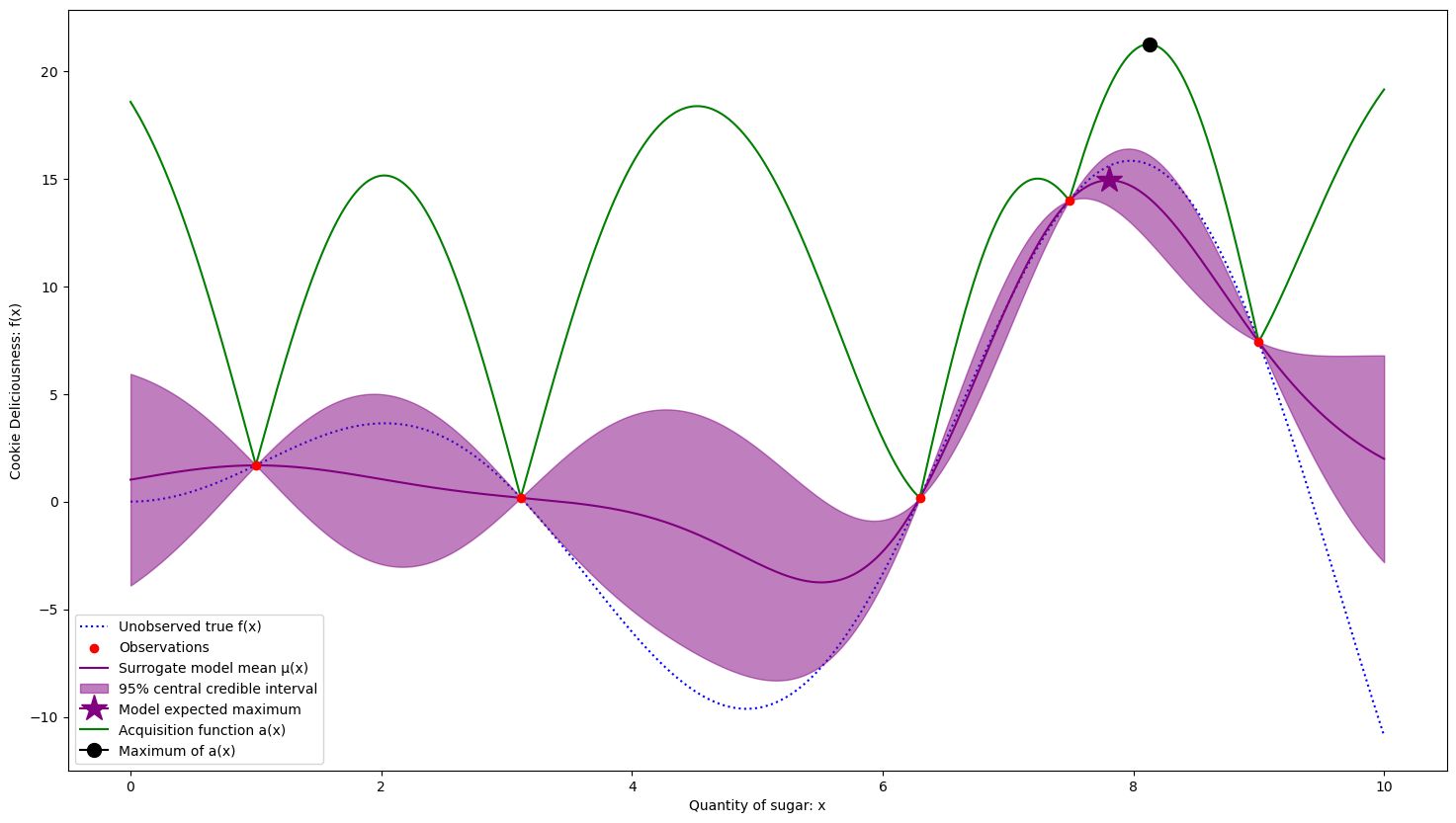
This continues until we concentrate around the best solution, after 9 samples.

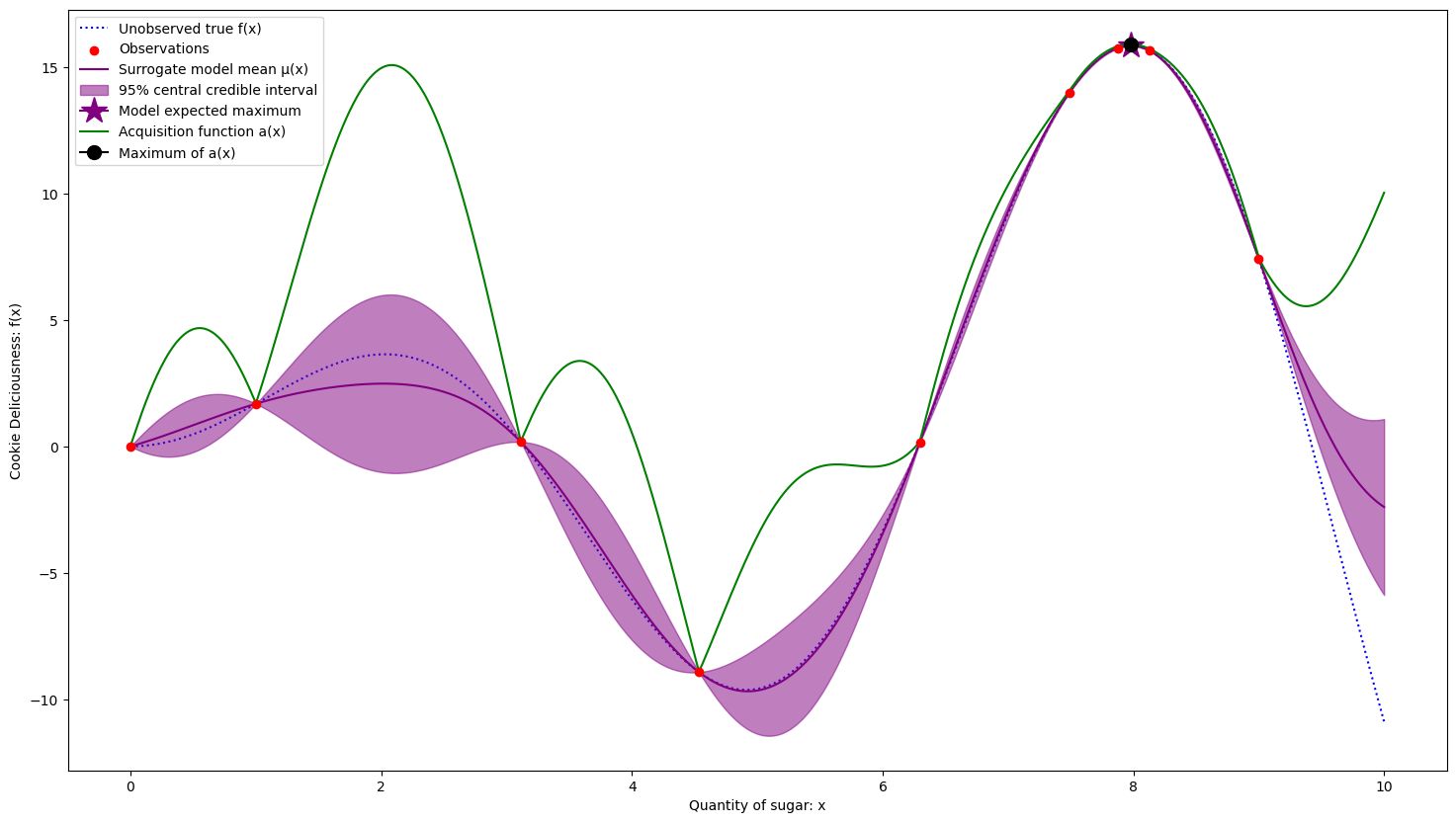
Global maximum estimated at x = 7.978 with f(x) = 15.833
True maximum at x = 7.978 with f(x) = 15.833

We were able to converge to the exact solution fairly quickly! Note how we sampled more in good regions, and have less uncertainty there. We are fine having uncertainty in areas that we don’t think will be as fruitful. This is due to the acquisition function which balances decreasing uncertainty with focusing on good regions. A good acquisition function will direct your optimization to learn only what it needs to in order to be confident in finding a good solution.

Acquisition function choice

There are many ways to pick an acquisition function, but something to keep in mind is that we want to balance exploration — searching for new points to decrease model variance; and exploitation — picking points that we expect will give optimal values.

Exploration

If we wanted to maximize exploration of the search space, we would want to pick the point that minimizes our total variance of the model. Here that would just be picking the value of $x$ where the model has the largest standard deviation $\sigma (x)$. Always pick the point with the widest interval.

$$\begin{array}{c}a(x)=\sigma (x)\end{array}$$

As you can see, it greatly reduces variance in the model but oversamples poor areas, undersamples good areas, and doesn’t converge. This would be a great way to characterise the function, but we are looking to optimize it in as few steps as possible.

Exploitation

We use the term exploitation to refer to how greedy a process is in selecting a solution that it thinks optimizes the problem. If we wanted to maximize exploitation, we would want to pick the point that maximizes expected $f$.

$$\begin{array}{c}a(x)=\mu (x)\end{array}$$

Here, we are lucky and we converge quickly to the best solution. However, you can see that many high variance regions of the search space are under-sampled. We could have easily fallen into a local maximum. This is sensitive to the initial sample of points.

Upper Confidence Bound

One intuitive way to balance exploration and exploitation is just to combine both of these terms. We can create an upper confidence bound with some value $\lambda$

$$\begin{array}{c}UCB(x)=\mu (x)+\lambda \sigma (x)\end{array}$$

and set this as our acquisition function. There are some nice theoretical properties to this function it’s effectiveness can be seen through this intuition about balancing the terms. Note when $\lambda =1.96$, the acquisition function is just the upper bound of the 95% interval.

For our initial acquisition function, we used UCB with $\lambda =7$

Other popular functions include Probability Improvement, Expected Improvement, Entropy Search, Predictive Entropy Search, and others. You can read about these in the literature.

Section 2 Recap

Bayesian Optimization is a framework for iteratively sampling a black-box function in order to find the global optimum. We don’t know the function directly, so we construct a model for the function because we can find the optimal value on the model. We choose samples through an acquisition function that balances exploration (reducing variance of the model) with exploitation (choosing areas where the model expects the solution to be good).

The BO algorithm is

1. Start with some initial sample measurements
2. Fit a probabilistic model to the data
3. Compute the acquisition function based on the model
4. Find $x^{\ast }$ that maximizes the acquisition function
5. Sample $f(x^{\ast })$ and add to your data
6. If time/resources are remaining, go to step 2

Sections 3 and 4 will cover Gaussian Processes and why we use them as our choice of model.